LandBrowser VNIR on GEE User’s guide

1. URL

https://landbrowser.users.earthengine.app/view/vnir

2. Purpose

LandBrowser VNIR visualizes globally mosaicked false color, true color and NDVI images generated every 3 months from top of atmosphere (TOA) reflectance observed by Landsat 9, Landsat 8, Landsat 7 (until June, 2003), and Landsat 5 (until May, 2012); Sentinel-2; Terra/ASTER data released from U. S. Geological Survey (USGS); European Space Agency (ESA); and National Aeronautics and Space Administration (NASA), Ministry of Economy, Trade and Industry (METI), National Institute of Advanced Industrial Science and Technology (AIST), and Japan Space Systems (JSS), respectively, on Earth Engine Apps.

3. Interface

The initial screen shows the latest false color image zoomed to Japan. The false color image is generated from satellite data observed in 3 months (January to March, April to June, July to September, and October to December of every year). The mosaicking processes are composed of simplified cloud masking and selecting median of TOA reflectance during the 3 months. Note that it could take a long time to show the false color image after you accessed the LandBrowser VNIR because several satellite scenes are used to generate mosaicked image. In addition, in erly January, April, July, and October, because the satellite observation is not enough, the false color image would be shown only in limited areas.

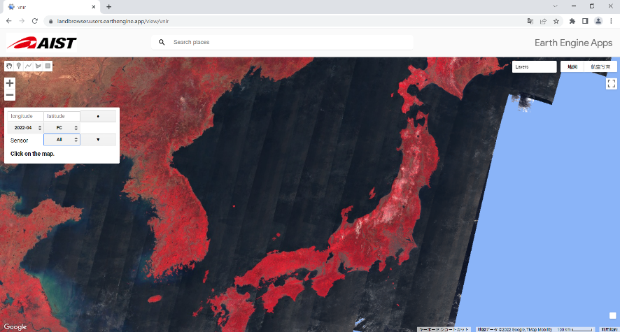
Fig. 1 Initial screen of LandBrowser VNIR.

To pan the map

• drag the map to a new place

• put a place name or map coordinate as longitude, latitude in the search box, and select a place from suggested candidates.

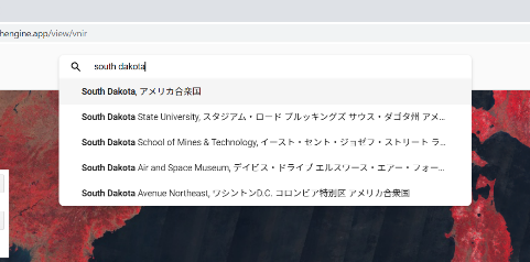
Fig. 2 Place name search.

• put longitude and latitude in the textboxes for coordinates and click the button.

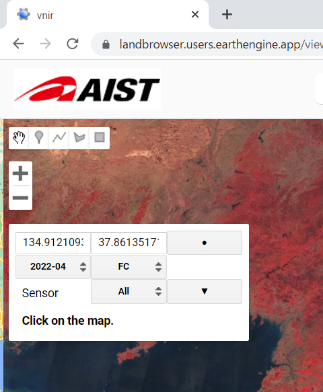
Fig. 3 Coordinate boxes.

To change zoom level, use mouse wheel or click + or - on the top-left on the screen.

Fig. 4 shows an example of displaying South Dakota, US accessed on June 29, 2022 (Note that the shown result depends on when you access the site).

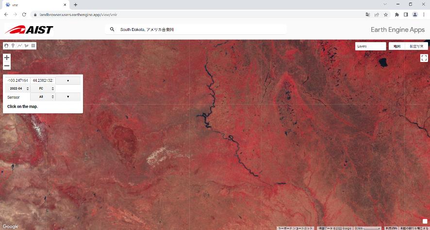
Fig. 4 False color image in South Dakota, US (accessed on June 29, 2022).

To change the period of image, select year-month from the pull-down menu.

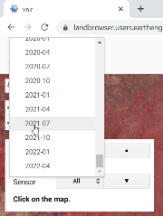
Fig. 5 Pull-down menu to select the period of image.

Fig. 6 shows false color image in South Dakota in July-September, 2021. In comparison with April-June, 2022 (Fig. 4), breadbasket in eastern side looks redder because of the grown crops.

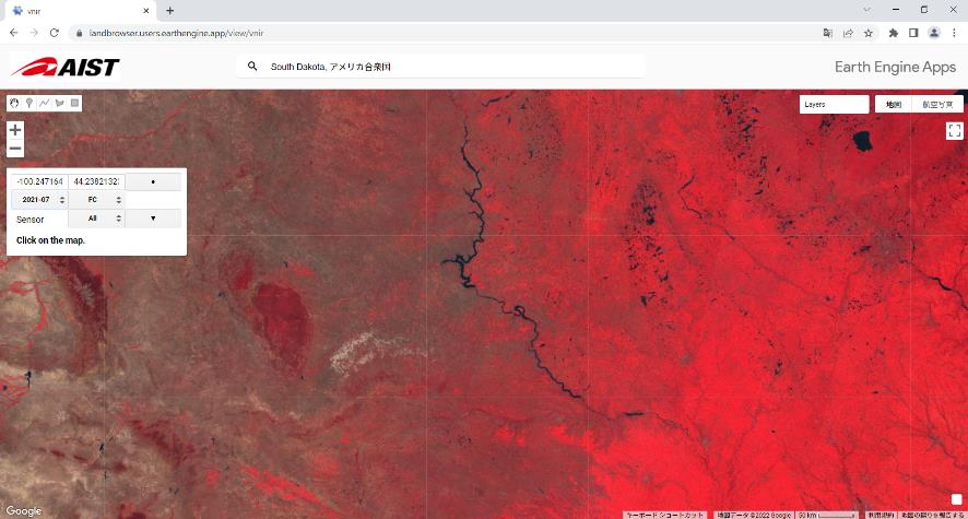
Fig. 6 False color image in South Dakota, US in July-September, 2021.

To check place name in the shown area, turn off the false color image by unchecking the checkbox of the layer to display underlying Google map layer.

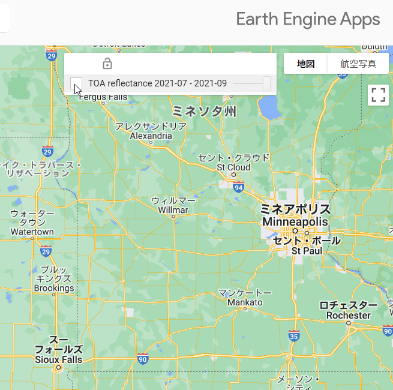
Fig. 7 Unchecking the checkbox of the layer of false color image.

You can select aerial photo instead of basemap as background.

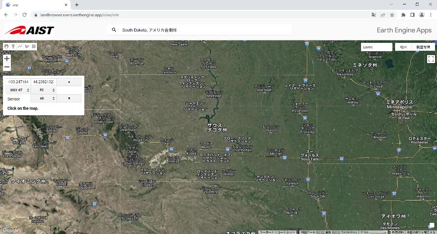
Fig. 8 Aerial photo as background.

You can select NDVI instead of false color image from the pull-down menu, which lists FC (false color) and NDVI.

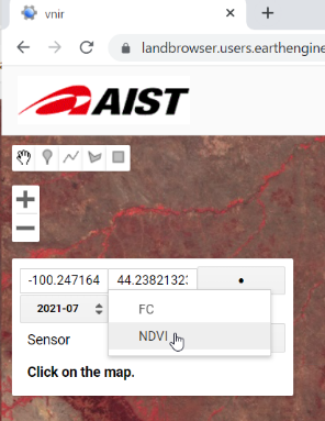
Fig. 9 Pull-down menu to select false color or NDVI.

Fig. 10 shows NDVI in South Dakota, US in July-September, 2021. Bottom right panel shows the legend for color of NDVI.

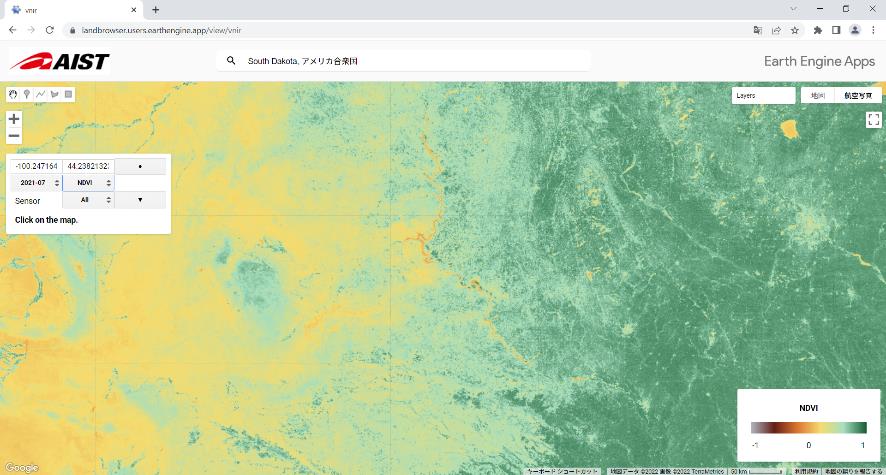
Fig. 10 NDVI in South Dakota, US in July-September, 2021.

Zooming into an area of interest (the central part) enhances the detailed view of the site. Fig. 11 and 12 show clear contast between planted and unplanted fields.

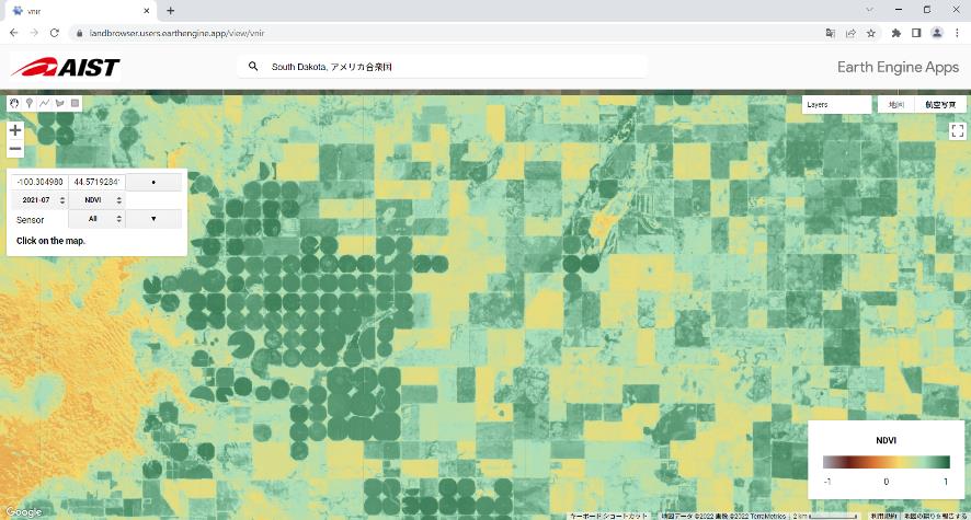
Fig. 11 NDVI in fields in South Dakota, US in July-September, 2021.

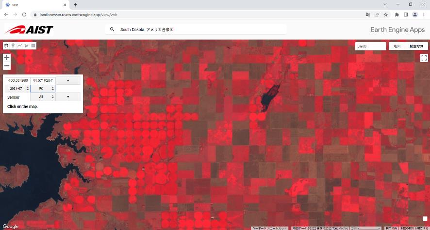
Fig. 12 False color image in fields in South Dakota, US in July-September, 2021.

4. Displaying individual satellite images

By clicking on the map, you can get the individual satellite images in the past over the clicked location. The latest false color image or NDVI, depending on which was selected, in the showing year is added along with a + marker at clicked point on the map. Additional dropdown menus to select the date of data acquisition and a graph to indicate timeseries TOA reflectance in Green (G), Red (R), and Near infrared (NIR) bands are shown on the left panel. Fig. 13 shows the false color image on June 27, 2022.

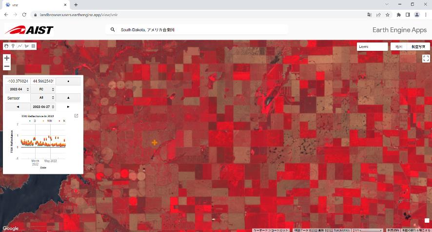
Fig. 13 False color image in fields in South Dakota, US on June 27, 2022.

To switch the date of data acquisition,

• select date from pull-down menu

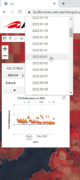
Fig. 14 Pull-down menu to select date of data acquisition date.

• click the point on the timeseries graph

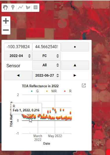
Fig. 15 Selecting data acquisition date from the timeseries graph.

• Click a button to change data acquisition date.

  • immediately before the currently showing date

  • immediately after the currently showing date

Fig. 16 shows the false color image on February 1, 2022 which was selected from the graph.

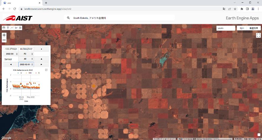
Fig. 16 False color image in fields in South Dakota, US on February 1, 2022.

The timesries graph plots annual change of TOA reflectance. To explore further past,

• select year-month from the pull-down menu (mosaicked image in selected period will be shown)

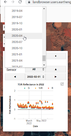
Fig. 17 Pull-down menu to select year and month of data acquisition date.

• then, click a button to show individual satellit image.

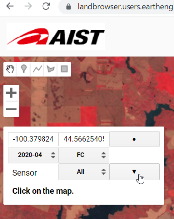
Fig. 18 Button to show individual satellit image.

Note that because cloud masking is not applied to individual satellite image, totally saturated image can be shown such as fields in South Dakota, US on December 29, 2020 shown in Fig. 19. Avoid selecting date with extremely high TOA reflectance, which is perhaps suffered from cloud coverage.

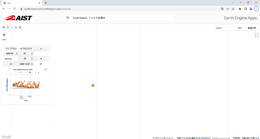
Fig. 19 False color image covered by cloud in fields in South Dakota, US on December 29, 2020.

Timeseries graph is corresponding to selected image type. Switch false color image to NDVI by selecting from pull-down menu and then click the button to show individual satellit image. Extremely low NDVI is possibly caused by cloud coverage (Fig. 20).

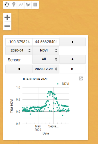
Fig. 20 Annual change of NDVI in a field in South Dakota, US in 2020.

5. Displaying satellite images taken by individual satellite sensor

When the individual satellite image is shown on the map, images taken by all satellite sensors are merged together over one day.

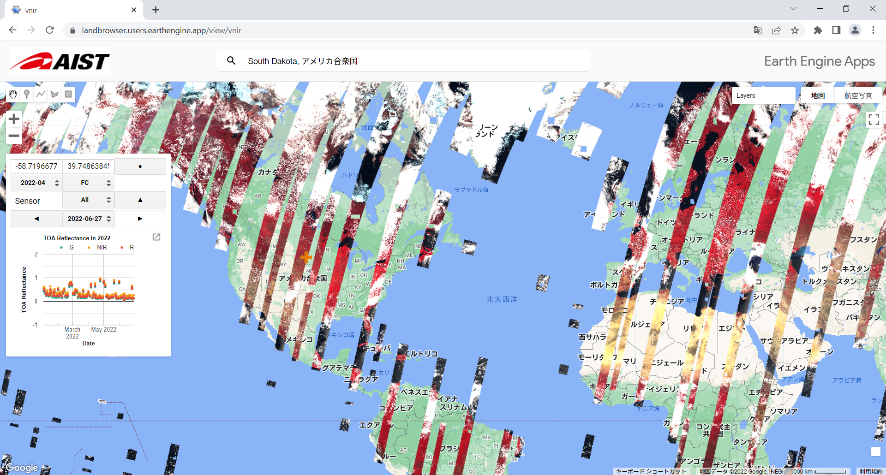
Fig. 21 Merged false color images taken by Landsat, Sentinel-2, and ASTER on June 27, 2022.

Fig. 22 is an example of merged images taken by Sentinel-2 (left) and Landsat 9 (right).

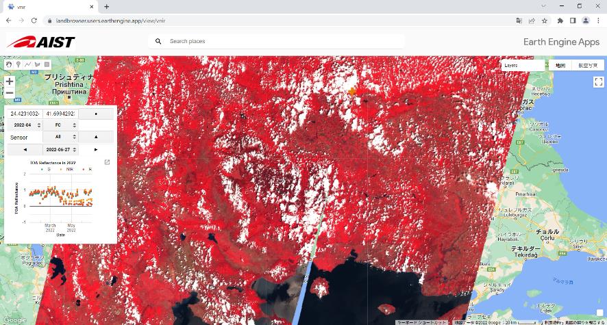
Fig. 22 Merged false color images taken by Sentinel-2 (left) and Landsat 9 (right) on June 27, 2022.

To show satellite image taken only by an individual satellite sensor, select satellite from “Sensor” pull-down menu, on which “All” is selected in default setting. Then click on the map or click the button to show/remove the individual satellite image twice.

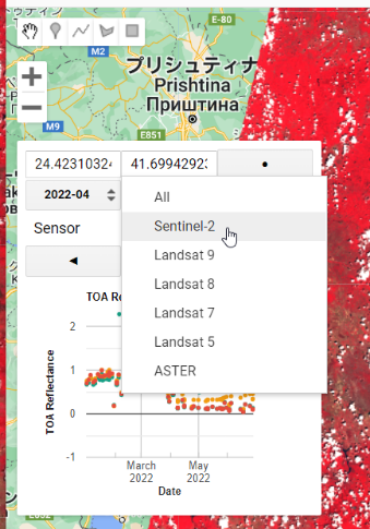
Fig. 23 Pull-down menu to select satellite sensor.

Fig. 24 shows the map only showing Sentinel-2 data on the location same as Fig. 22. When Sentinel-2 was selected, timeseries graph shows TOA reflectance in Blue (B), G, R, NIR, Shortwave infrared (SW1: 1.6 micron) and Shortwave infrared (SW2: 2.2 micron) instead of only G, R, and NIR.

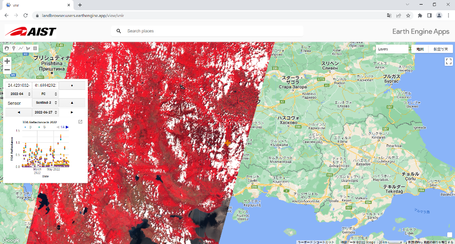
Fig. 24 False color images taken by Sentinel-2 on June 27, 2022.

Tale below shows the band numbers to be shown in the timeseries TOA reflectance graph.

	All	Sentinel-2	Landsat 8/9	Landsat 5/7	ASTER
Blue (B)	No	Band 2	Band 2	Band 1	No
Green (G)	yes	Band 3	Band 3	Band 2	Band 1
Red (R)	yes	Band 4	Band 4	Band 3	Band 2
Near infrared (NIR)	yes	Band 8A	Band 5	Band 4	Band 3N
Shortwave infrared 1 (SW1)	No	Band 11	Band 6	Band 5	No
Shortwave infrared 2 (SW2)	No	Band 12	Band 7	Band 7	No

6. Downloading a timeseries plot

You can download the timeseries plot.

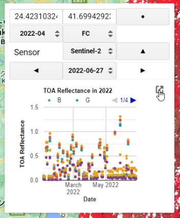
Fig. 25 Button to open the plot in the new tab.

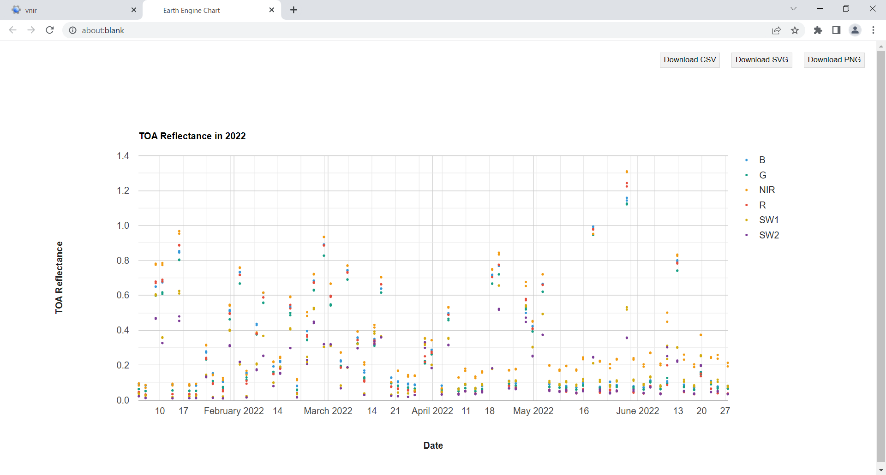
Fig. 26 The timeseries plot in the new tab.

By clicking the buttons in the upper right, you can save the plotted data in CSV format and the plot as images in SVG or PNG formats.

7. Permalink

Click “Get URL” button to construct a permalink corresponding to the current status of the maps. You can revisit the current map by accessing the URL in the address bar. For example, the URL for the map in Fig. 24 is https://landbrowser.users.earthengine.app/view/vnir#lon=24.4231032;lat=41.6994292;zoom=8;date=2022-06-27;ym=2022-04;layer=FC;sat=Sentinel-2; .

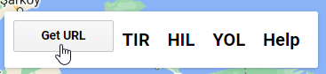
Fig. 27 Button to get permalink to the current status of the maps.

8. Links to the other LandBrowsers

The links of “TIR”, “HIL” and “YOL” take you to LandBrowser TIR , Hotarea-hil and Hotarea-yol , respectively, with the current status of the map. We recommend you to click “Get URL” button before clicking these links to make sure the latest status of the map.

Fig. 28 The links to open the other LandBrowser apprications.

9. Terms of use

The terms of use follows those of Google Earth Engine.

Reference

1

TBD